Logistic Regression with TensorFlow

In the previous post we’ve seen the basics of Logistic Regression & Binary classification.

Now we’re going to see an example with python and TensorFlow.

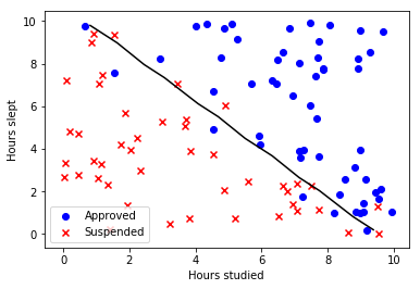
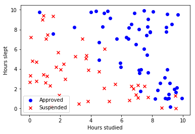
On this example we’re going to use the dataset that shows the probability of passing an exam by taking into account 2 features: hours studied vs hours slept.

First, we’re going to import the dependencies:

1
2
3
4
5
6
7
8
# Import dependencies
import numpy as np
import matplotlib.pyplot as plt
import tensorflow as tf
import sklearn
from sklearn.model_selection import train_test_split

%matplotlib inline
1
2
3
4
5
6
7
8
9
10
11
12
13
14
15
16
17
18
19
20
21
22
23
24
25
26
27
28
data = np.genfromtxt('data_classification.csv', delimiter=',')

#Get the 2 features (hours slept & hours studied)
X = data[:, 0:2]
# Get the result (0 suspended - 1 approved)
Y = data[:, 2]


# Plotting
pos = np.where(Y == 1)
neg = np.where(Y == 0)
plt.scatter(X[pos, 0], X[pos, 1], marker='o', c='b')
plt.scatter(X[neg, 0], X[neg, 1], marker='x', c='r')
plt.xlabel('Hours studied')
plt.ylabel('Hours slept')
plt.legend(['Approved', 'Suspended'])
plt.show()

#Split the data in train & test
Y_reshape = data[:,2].reshape(data[:,2].shape[0], 1)
x_train, x_test, y_train, y_test = train_test_split(data[:, 0:2], Y_reshape)

print ("x_train shape: " + str(x_train.shape))
print ("y_train shape: " + str(y_train.shape))
print ("x_test shape: " + str(x_test.shape))
print ("y_test shape: " + str(y_test.shape))

num_features = x_train.shape[1]

Now we’re building the logistic regression model with TensorFlow:

1
2
3
4
5
6
7
8
9
10
11
12
13
14
15
16
17
18
19
20
21
22
23
24
25
26
27
28
29
30
31
32
33
34
35
36
37
38
39
40
41
42
43
44
learning_rate = 0.01
training_epochs = 1000

tf.reset_default_graph()

# By aving 2 features: hours slept & hours studied
X = tf.placeholder(tf.float32, [None, num_features], name="X")
Y = tf.placeholder(tf.float32, [None, 1], name="Y")

# Initialize our weigts & bias
W = tf.get_variable("W", [num_features, 1], initializer = tf.contrib.layers.xavier_initializer())
b = tf.get_variable("b", [1], initializer = tf.zeros_initializer())

Z = tf.add(tf.matmul(X, W), b)
prediction = tf.nn.sigmoid(Z)

# Calculate the cost
cost = tf.reduce_mean(tf.nn.sigmoid_cross_entropy_with_logits(logits = Z, labels = Y))

# Use Adam as optimization method
optimizer = tf.train.AdamOptimizer(learning_rate).minimize(cost)

init = tf.global_variables_initializer()

cost_history = np.empty(shape=[1],dtype=float)

with tf.Session() as sess:
sess.run(init)

for epoch in range(training_epochs):
_, c = sess.run([optimizer, cost], feed_dict={X: x_train, Y: y_train})
print("Epoch:", '%04d' % (epoch+1), "cost=", "{:.9f}".format(c), \
"W=", sess.run(W), "b=", sess.run(b))
cost_history = np.append(cost_history, c)


# Calculate the correct predictions
correct_prediction = tf.to_float(tf.greater(prediction, 0.5))

# Calculate accuracy on the test set
accuracy = tf.reduce_mean(tf.to_float(tf.equal(Y, correct_prediction)))

print ("Train Accuracy:", accuracy.eval({X: x_train, Y: y_train}))
print ("Test Accuracy:", accuracy.eval({X: x_test, Y: y_test}))

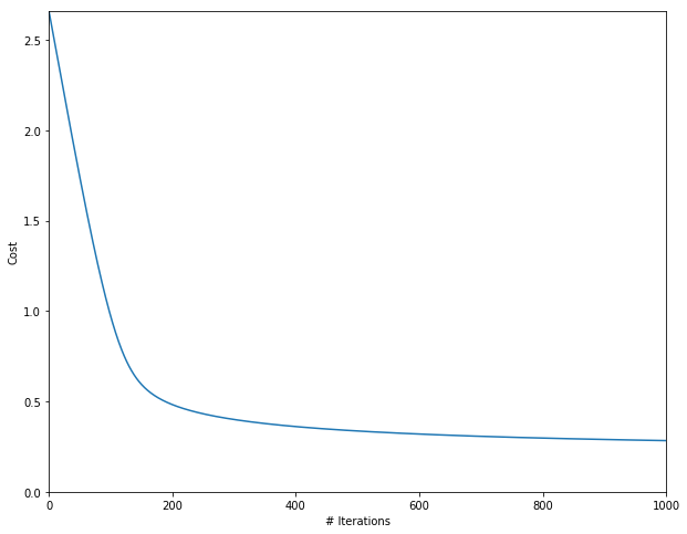
Our accuracy is 86% not too bad with a dataset of only 100 elements. The optimization of the cost function is as follows:

So, our linear regression example looks like follows:

Share Comments